
An example of \(\psi\).
Notes on getting a veering triangulation from a pseudo-Anosov flow
16.06.2026These notes follow [Farb–Margalit], [Landry–Minsky–Taylor], [Barthelmé–Mann] and [Tsang].
Let \(f \in \text{Mod}(T^2)\). We say that \(f\) is Anosov if there is an affine representative \(\psi \in f\) and a pair of measured foliations \((\mathcal{F}^s, \mu_s)\) and \((\mathcal{F}^u, \mu_u)\) on \(T^2\) such that
An example of \(\psi\).
The animation above shows an example of the map \(\psi = \begin{pmatrix}2&1\\1&1\end{pmatrix}\). The third condition in the definition above is saying that the map \(\psi\) should stretch along \(\color{green}\mathcal{F}^u\) and compress along \(\color{purple}\mathcal{F}^s\). In the animation, we can see the green foliation stretching and the purple foliation compressing. The associated mapping class \([\psi]\) is an exmaple of an Anosov mapping class. Some simple linear algebra shows that \(f\) is Anosov if and only if the associated matrix \(A \in \text{SL}_2(\mathbb Z)\) has trace with absolute value greater than 2. In fact, it's easy to classify the elements of \(\text{Mod}(T^2)\) by the number of distinct real eigenvalues of the associated matrix, but we won't need that for these notes.
We would like to mimic Anosov maps on higher genus surfaces, but we're quicky foiled by the Poincaré–Hopf Theorem, which obstructs the existence of foliations on higher genus surfaces. All we have to do, though, is allow singular foliations, hence the "pseudo". A pseudo-Anosov map is the same as an Anosov map, but we require \(\mathcal{F}^s\) and \(\mathcal{F}^u\) to have at least one singular point.

A pseudo-Anosov map near a 3-pronged singularity.
Most of what I say in this section can be extended to compact surfaces, but things are easier to state for closed surfaces.
Let \(S\) be a closed surface of genus \(g \geq 2\), and let \(\psi\) be a pseudo-Anosov homeomorphism on \(S\). Let \(\mathcal F\) be either the stable or unstable foliation of \(\psi\). Any leaf \(L\) of \(\mathcal F\) is either stretched or compressed, but never both. If \(L\) were closed (i.e. an embedded circle), then we would have a continuous map on the circle which expands everywhere or contracts everywhere, which isn't possible. For the same reason, \(L\) can't connect two singular points of the foliation. Thus we get the following:
Lemma. If \(L\) is any leaf of the (un)stable foliation of a pseudo-Anosov map \(\psi\) on a closed surface \(S\), then \(L\) is neither closed nor connects two singular points.
We can say more about the leaves.
Theorem. (Poincaré Recurrence) Let \((\mathcal F, \mu)\) be a measured foliation on compact \(S\). Let \(L\) be an infinite half-leaf. Then any arc transverse to \(\mathcal F\) and intersecting \(L\) must intersect \(L\) infintely often.
A proof for this can be found in [Farb–Margalit]. It relies on the strong property that measured foliations on surfaces admit so-called "good" atlases. As a result, we get a nice decomposition of the surface into rectangles which play nicely with the (un)stable foliation:
Construction. (Rectangle Decomposition) Let \(\mathcal F\) be the (un)stable foliation of a pseudo-Anosov homeomorphism \(\psi\). Let \(\alpha\) be any curve transverse to \(\mathcal F\), and assume that if \(\alpha\) intersects a singularity, it does so at most once and at an endpoint. We will subdivide \(\alpha\) by adding a finite number of vertices onto \(\alpha\) in the following ways:
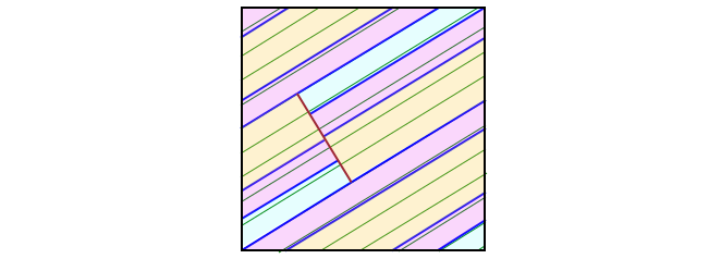
A rectangle decomposition of the Anosov map given in the first section above with the chosen curve \(\alpha\) in red. There are three rectangles.
Let \(\alpha\) be an arbitrary curve transverse to \(\mathcal F\) as above, and let \(\mathcal R\) be its rectangle decomposition. Pick any leaf \(L\) in the foliation. Well, since \(L\) is at least half-infinite (by the Lemma above), and since \(L\) must live in some rectangle \(R \in \mathcal R\), the leaf \(L\) must hit an edge of \(R\) which is transverse to \(\mathcal F\). But all such edges lie by construction in \(\alpha\). Thus, \(L\) (which we chose arbitrarily!) must intersect \(\alpha\). We thus get the following corollary.
Corollary. Let \(\mathcal F\) be the (un)stable foliation of a pseudo-Anosov homeomorphism on a closed surface \(S\). Then every leaf is dense in \(S\).
Consider the orbit of a point \(x\in S\) under a pseudo-Anosov homeomorphism \(\psi\), i.e. the set \(\{\psi^n(x)\:|\:n\in\mathbb Z\}\). This will become important when we start considering flows in the next section, but the dynamics of pseudo-Anosov maps are also of independent interest. It's important to note that we are not quotienting our homeomorphisms by isotopy (c.f. there are representatives of periodic mapping classes with non-periodic orbits). Are there points with dense orbit? What points have finite orbit? The following theorem answers the first question.
Theorem. Let \(\psi\) be an orientation preserving pseudo-Anosov homeomorphism of a closed surface \(S\). Then there is a point \(x\in S\) for which \(\psi\) has a dense orbit.
Proof. By taking a power of \(\psi\), we may assume without loss of generality that \(\psi\) fixes the singular points of
the foliations (note this isn't necessarily the case: one can imagine composing a pseudo-Anosov mapping class with a periodic
mapping class and taking an appropriate representative homeomorphism which permutes the singular points of the foliation).
We'll first show that a nonempty open set \(U \subset S\) which is set-wise invariant under \(\psi\) must be dense.
If \(U\) is such a set, then a leaf of the stable foliation with one end on a singular point \(s\) must intersect \(U\) by the fact
that leaves are dense (above lemma). So there is a point \(x\in U\) which lies on such a leaf. Let \(J \subset U\) be a segment
of the leaf of the unstable foliation which contains \(x\).
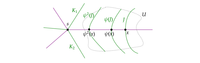
Now let \(\{U_i\}\) be a countable basis for \(S\), and define \(V_i = \bigcup_{n\in\mathbb Z} \psi^n(U_i)\). Each \(V_i\) is nonempty, open, and invariant under \(\psi\), so each \(V_i\) is dense in \(S\). Thus \(\bigcap_i V_i\) is dense in \(S\) by the Baire Category Theorem. We only really need that this set is nonempty. So take \(x \in \bigcap_i V_i\), and observe that \(x \in \psi^n(U_i)\) for some \(n\) but for all \(i\). In other words, for every basis element \(U_i\), there is an \(n\) for which \(\psi^{-n}(x) \in U_i\). Since every basis element contains an element of the orbit of \(x\), we get that every open set in \(S\) contains an element of the orbit of \(x\). Thus, the orbit of \(x\) is dense in \(S\). \(\;\;\;\Box\)
Now we'll consider points with periodic orbit. For instance, every singular point of the (un)stable foliation has a periodic orbit. In the first section of these notes, I animated an Anosov (but not pseudo-Anosov) map on the torus, where the "origin" is fixed, and thus has periodic orbit. Actually for any linear Anosov map of the torus, the image of \(\mathbb Q^2\) under the projection \(\mathbb R^2 \to T^2\) has periodic orbit, and thus is dense in \(T^2\). The following theorem says this holds more generally.
Theorem. If \(\psi\) is a pseudo-Anosov homeomorphism on a compact surface \(S\), then the periodic points of \(\psi\) are dense in \(S\).
A proof can be found in [Farb–Margalit].
Let \(N\) be a closed, orientable 3-manifold. It's useful to study \(N\) by the flows it admits. We'll take a flow to be a continuous map \(\phi^t \::\: N\times \mathbb R \to N\). However, we will only consider flows up to orbit equivalence so that we can ignore details about specific parametrizations. If \(N\) is a surface bundle over the circle, then there is an obvious flow given by taking the unit tangent in the circle direction. Such a flow is called a suspension flow. If \(N\) is a surface bundle whose monodromy is a pseduo-Anosov map \(\psi\), then the properties of the definitions in the previous section tell us something about the manifold.
The goal now is to mimic the behavior of suspension flows of pseudo-Anosov maps on general closed manifolds (which are not necessarily mapping tori of pseudo-Anosov homeomorphisms). For technical reasons, we will restrict to considering trasitive flows, which are flows with a dense orbit. This is not a strong restriction.
Let \(\phi_{n,k,\lambda}\) be the lift of the map \(\begin{pmatrix}\lambda&0\\0&\lambda^{-1}\end{pmatrix}\) over the semi-branched cover \(z\mapsto z^{n/2}\) followed by a rotation of \(2\pi k/n\). A pseudo-hyperbolic orbit \(\Phi_{n,k,\lambda}\) is the mapping torus of the semi-branched cover of the map \(\phi_{n,k,\lambda}\) on a neighborhood of the origin. The animation at the end of the first section is a rising cross-section of the mapping torus \(\Phi_{3, 0, 1/2}\). This induces two-dimensional foliations \(\Lambda^u\) and \(\Lambda^s\), illustrated below.
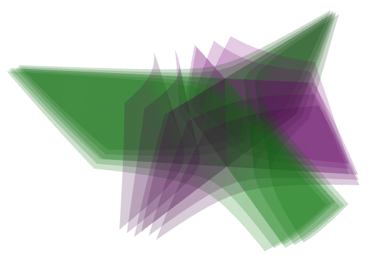
The 2D foliations \(\Lambda^u\) and \(\Lambda^s\) near a singularity. You can interact with the image here or with lower opacity here.
A pseudo-Anosov flow on a closed, orientable 3-manifold \(N\) is a continuous flow such that
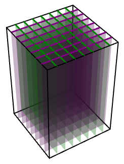
A flow box. You can interact with the image here.
Condition 5 is supposed to mimic the compress/stretch behavior of the suspensions of \(\mathcal F^s\) and \(\mathcal F^u\) corresponding to a pseudo-Anosov map.
Let \(\phi\) be a pseudo-Anosov flow on a closed 3-manifold \(N\). Lift \(\phi\) to the universal cover \(\widetilde N\) to get a flow on \(\widetilde N\). The orbit space \(\mathcal O\) is the set of orbits of \(\widetilde \phi\) endowed with the quotient topology.
We remark that if \(N\) is a mapping torus of a pseudo-Anosov homeomorphism \(\psi :S\to S\) and \(\phi\) is the corresponding suspension flow, then the orbit space of \(\phi\) is \(\widetilde S\).
Theorem. \(\mathcal O\) is homeomorphic to \(\mathbb R^2\). Moreover, \(\Lambda^s\) and \(\Lambda^u\) project to (possibly singular) one-dimensional foliations \(\mathcal O^s\) and \(\mathcal O^u\) under the quotient \(\widetilde N \to \mathcal O\).
A perfect fit rectangle \(R\) in \(\mathcal O\) is a properly embedded copy of \([0,1]^2\setminus \{(1,1)\}\) such that the vertical
and horizonal foliations of \(R\) are sent to \(\mathcal O^s\) and \(\mathcal O^u\).
A perfect fit rectangle.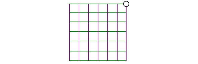
Let \(C\) be a nonempty finite collection of closed orbits of \(\phi\) which includes all singular orbits of \(\phi\). Let \(\widetilde C\) be the set of orbits of \(\widetilde\phi\) which cover the orbits in \(C\). We will also use \(\widetilde C\) to refer to the image of \(\widetilde C\) under the quotient \(\widetilde N \to \mathcal O\) when context makes it clear. We say \(\phi\) has no perfect fits relative to \(C\) if there are no perfect fit rectangle in \(\mathcal O\) disjoint from \(\widetilde C\). If \(\phi\) has no perfect fits relative to the set of singular orbits, then \(\phi\) has no perfect fits . Despite the verbiage, the case where \(\phi\) has no perfect fits is the good case.
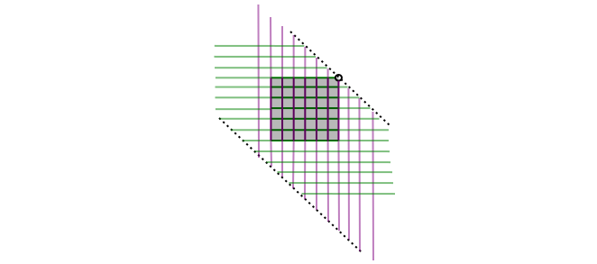
The "bad" case, where \(\mathcal O\) (homeomorphic to \(\mathbb R^2\)) contains a perfect fit rectangle (highlighted).
Lemma. Let \(\phi\) be a transitive pseudo-Anosov flow on a closed 3-manifold \(N\). There exists a collection of orbits \(C\) such that \(\phi\) has no perfect fits relative to \(C\). Moreover, \(C\) can be chosen to be the set of singular orbits plus one other orbit.
A proof for this fact can be found in [Tsang].
We will also need the notion of the completed flow space \(P\), defined to be the infinite branched cover of \(\mathcal O\) over \(\widetilde C\). In other words, take the universal cover of \(\mathcal O \setminus \widetilde C\) and "put the set \(\widetilde C\) back in place". Note that \(\mathcal O^{s}\) and \(\mathcal O^{u}\) lift to foliations \(P^s\) and \(P^u\).
Let \(M\) be the cusped manifold given by cutting out the set of closed orbits \(C\) from \(N\). There is an induced flow \(\hat\phi\) on \(M\). We summarize relationship between these objects in the following diagram.
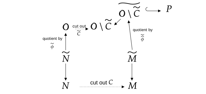
The characters at play.
Observe that the action of \(\pi_1(M)\) on \(\widetilde M\) respects the orbits of \(\widetilde{\hat\phi}\), and thus induces an action of \(\pi_1(M)\) on \(P\). This action will be useful in the next section.
Lastly, we will say a rectangle in \(P\) is an embedding of \([0,1]^2\) in \(P\) such that \(P^s\) and \(P^u\) are conjugate to the foliation by horizontal and vertical lines, and such that no branch point of \(P\) lies in the interior of \(R\). A rectangle \(R_2\) is taller than \(R_1\) if every leaf of \(P^u\) intersecting \(R_1\) also intersects \(R_2\). Similarly, \(R_2\) is wider than \(R_1\) if every leaf of \(P^s\) intersecting \(R_1\) also intersects \(R_2\).
We now construct a veering triangulation when given a pseudo-Anosov flow, as stated more carefully in the theorem below. This construction is due to Agol and Guéritaud around 2015, with Landry, Minsky, and Taylor upgrading their statement to the one below in 2021.
Theorem. Let \(\phi\) be a pseudo-Anosov flow with no perfect fits relative to a set \(C\). Then there exists a veering triangulation \(\Delta\) on \(N\setminus C\) such that \(\phi\) is positively transverse to the 2-skeleton of \(\Delta\).
Before we prove this, we introduce some notation. Let \(S\) be the set of branch points in \(P\). An edge rectangle is a rectangle in \(P\) with opposite corners on distinct elements of \(S\). A face rectangle is a rectangle in \(P\) with one corner on \(S\) and one element of \(S\) on each edge opposite that corner. A tetrahedron rectangle is a rectangle with one element of \(S\) on each of its edges. Observe that due to condition 5 in the definition of a pseudo-Anosov flow, the points of \(S\) in each tetrahedron rectangle cannot have the same x-coordinate or the same y-coordinate.

Left to right: edge rectangle, face rectangle, tetrahedron rectangle.
For each rectangle in \(P\), there is a sensible, consistent choice of cardinal directions. If the elements of \(S\) in an edge rectangle lie on the NE and SW corners, then we call it a red edge and say that it's right veering. If the elements of \(S\) lie on the NW and SE corners, then we call it a blue edge and say that it's left veering.

A blue edge rectangle and a red edge rectangle.
Lemma. There are finitely many edge rectangles in \(P\), up to the action of \(\pi_1(M)\).
Proof. First note that at every branch point \(s \in S\), there are countably many leaves of \(P^s\) and \(P^u\)
which intersect \(s\), as in the figure below. Two such leaves \(L_1\) and \(L_2\) are adjacent if \(P\setminus(L_1\cup L_2)\)
has a component with no leaves of \(P^s\) or \(P^u\) intersecting \(s\). Such a component \(\Omega\) is called an orthant. Thus an
orthant has one leaf of \(P^s\) and one leaf of \(P^u\) as boundary. The point \(s\) is the corner singularity of \(\Omega\).
Part of a neighborhood of a singularity \(s\) (red) in \(P\) and
the leaves of the foliation which intersect \(s\). You can interact
with the image here.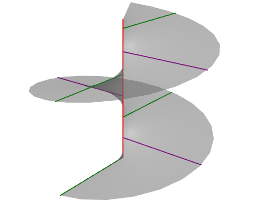
The staircase \(A\) corresponding to \(\Omega\) is the set of all edge rectangles in \(\Omega\) with one corner on its corner singularity.
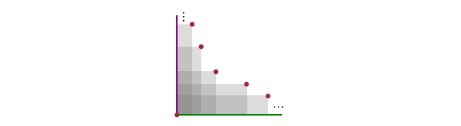
A staircase inside an orthant.
Let \(E\) be the set of edge rectangles in \(A\). There is a natural ordering on \(E\) (given in the picture above by the height of each rectangle). The action of any element \(g\in\text{Stab}(\Omega)\) must maintain this ordering, and thus the stabilizer of \(\Omega\) is cyclic.
Now, since \(\Gamma\) is finite, there are finitely many points of \(S\) up to the action of \(\pi_1(M)\). It follows that there are finitely many orthants in \(P\) up to the action of \(\pi_1(M)\). Since the stabilizer of each orthant is cyclic (and order-preserving cyclic actions on \(\mathbb Z\) are cofinite), there are finitely many edge rectangles up to the action of \(\pi_1(M)\). \(\;\;\;\;\Box\)
Now we return to the theorem. We will prove a weaker version of what was stated at the beginning of this section, and the remaining claims can be found in [LMT].
Theorem. Let \(\phi\) be a pseudo-Anosov flow with no perfect fits relative to a set \(C\). Then there exists a veering triangulation \(\Delta\) on \(M=N\setminus C\).
Proof. Let \(P\) be the complete orbit space of \(\phi\), and associate to each tetrahedron rectangle \(R\) in \(P\) a taut ideal tetrahedron \(t_R\) as determined by the edge rectangles contained in \(R\). The edges with a \(\pi\) angle are the ones with endpoints on opposite edges of \(R\). The orientation of \(\phi\) determines a transverse direction of the tetrahedra. We can then glue these (combinatorial) tetrahedra together along their shared faces to get a triangulation \(\widetilde \Delta\) of some new topological space \(\widetilde T\).
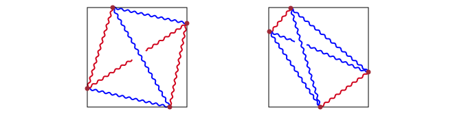
Two possibilites of associating a taut tetrahedron to a tetrahedron rectangle. Following [LMT], the wavy lines emphasize that there is no canonical way to embed them.
Since the action of \(\pi_1(M)\) on \(P\) preserves edge, face, and tetrahedron rectangles, \(\pi_1(M)\) acts simplicially and cofinitely (by the previous lemma) on \(\widetilde \Delta\). Note that the stabilizers of singularities in \(P\) correspond to the peripheral subgroups of \(\pi_1(M)\). Since the peripheral subgroups intersect pairwise trivially, \(\pi_1(M)\) acts properly discontinuously on \(\widetilde T\) (for if an element \(g\in\pi_1(M)\) fixed an edge, face, or tetrahedron, \(g\) would fix more than one singularity, and thus would be in the intersection of two peripheral subgroups, and thus would be the identity). From this, we get that \(T = \widetilde T / \pi_1(M)\) is an irreducible manifold, and \(\Delta = \widetilde \Delta / \pi_1(M)\) is a triangulation of \(T\). Observe that \(\Delta\) is veering by construction.
What's left to show is that \(T \cong M\). For this, we use the following result of Waldhausen:
Lemma. ([Waldhausen, Cor. 6.5]) Let \(M\) and \(T\) be manifolds which are irreducible and boundary-irreducible. Suppose \(M\) is sufficiently large. Let \(\psi\::\pi_1(T) \to \pi_1(M)\) be an isomorphism which respects the peripheral structure. Then there exists a homeomorphism \(f: T\to M\), which induces \(\psi\).
Note that \(\widetilde T\) is contractible and homotopy equivalent to \(\widetilde M\). It follows that \(\pi_1(T)\) is isomorphic to \(\pi_1(M)\). By the comments on peripheral subgroups above, \(M\) and \(T\) satisfy the conditions of the hypothesis in the lemma above, so we are done. \(\Box\)